

Concepts: Graphical method and the corner point method
Linear Programming22 min readLesson 3 of 6
3.1 Drawing the feasible region
The graphical method turns the constraints into picture. Each linear inequality in x and y defines one side of a straight line, so the set of points satisfying all of them is the common part of several half planes. Draw each boundary line, decide which side satisfies the inequality, and shade the common region. That shaded polygon is the feasible region, and every point inside it or on its boundary is a feasible solution.
The boundary lines are found from the corresponding equations: replace the inequality sign by an equals sign and draw that line through its two intercepts. A quick test point, usually the origin, decides which side satisfies the inequality. For a less-than constraint the region generally contains the origin unless the constant is negative; for a greater-than constraint it generally lies away from the origin. The non-negativity constraints keep the region in the first quadrant.
The feasible region of a linear programming problem is always convex, which is why its corners are so useful. It may be bounded, meaning it fits inside a circle, or unbounded, meaning it extends forever in some direction. The points where two boundary lines meet on the boundary of the region are its corner points, or vertices.
3.2 The corner point method
The theorem that makes the method work says that an optimal value, if it exists, must occur at a corner point. When the region is bounded, both a maximum and a minimum exist and each is reached at a corner. So the method reduces to three steps: list the corner points, evaluate the objective at each of them, and read off the largest and smallest values.
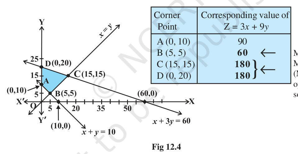
If two corner points give the same optimal value, then the whole segment joining them is optimal as well, so the problem has infinitely many optimal solutions. The exercises include this case: a minimum of 60 is obtained at two different corners, and every point on the edge between them also gives 60.
3.3 Unbounded regions and half-plane tests
An unbounded feasible region needs one extra step. The corner values are only candidates now, because the objective may improve without limit as the region extends. To test a candidate maximum M from the corner values, draw the line ax plus by equals M and check whether the half plane ax plus by greater than M has any point in common with the feasible region. If it does, the objective can be pushed beyond M and there is no maximum. If it does not, M is the maximum. The minimum is tested in the same way with the half plane below the candidate value.
A separate outcome is a problem with no feasible region at all. If the half planes have no common point, there is no feasible solution and the problem has no answer, whatever the objective. That situation is tested once in the chapter and appears in board papers as a straight question about the existence of a solution.
3.4 Worked examples
Example 1. For Z = 4x + y, take the constraints x + y at most 50, 3x + y at most 90, with non-negativity. The corner points are (0, 0), (30, 0), (20, 30) and (0, 50). The values of Z are 0, 120, 110 and 50, so the maximum is 120 at (30, 0).
Example 2. For Z = 200x + 500y, take the constraints x + 2y at least 10, 3x + 4y at most 24, with non-negativity. The corners are (0, 5), (4, 3) and (0, 6), with values 2,500, 2,300 and 3,000. The minimum is 2,300 at (4, 3).
Example 3. Take Z = 3x + 9y with x + 3y at most 60, x + y at least 10 and x at most y, together with non-negativity. The corners are (0, 10), (5, 5), (15, 15) and (0, 20), with values 90, 60, 180 and 180. The minimum is 60 at (5, 5), and the maximum is 180, reached at both (15, 15) and (0, 20). Because two corners give the same maximum, every point on the segment joining them is also optimal.
Slideshow, slide 1 of 3. Use the left and right arrow keys to change slides and the space bar to play or pause.
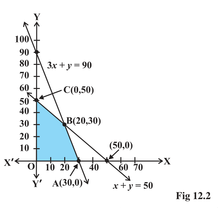
The shaded feasible region OABC for a two-variable linear programming problem, with its corner points marked.
3.5 When there is no solution
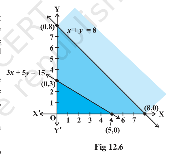
Example 4. For Z = 3x + 2y, take the constraints x + y at least 8, 3x + 5y at most 15, with non-negativity. The two constraints point in opposite directions: the first needs large x and y while the second allows only a small region near the origin. The half planes do not meet, so there is no feasible region and the problem has no feasible solution.
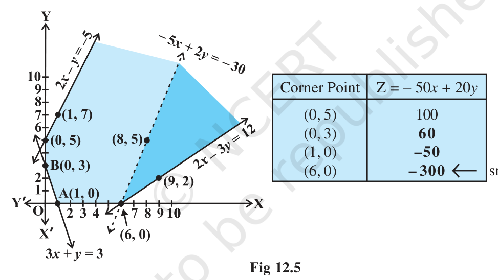
Example 5. Determine the minimum of Z = -50x + 20y subject to 2x - y at least -5, 3x + y at least 3, 2x - 3y at most 12, x, y at least zero. The feasible region is unbounded. The smallest corner value is -300 at (6, 0), but the half plane -50x + 20y less than -300 turns out to contain points of the feasible region, so the objective can fall below -300 and the problem has no minimum.
Exam
A graphical solution earns marks for the correct shading, the correctly labelled corner points and the evaluation table. Write the corner values in a small table with the objective value beside each point, and finish with a sentence that names the optimal point and value. For an unbounded region, the half-plane test is a separate mark, so do not leave it out.
Common mistake
Do not test only one or two corners and stop; list every corner of the feasible region. Do not accept the largest corner value as the maximum when the region is unbounded without the half-plane test. And do not draw the region with the wrong inequality direction: always check one test point.