

Concepts: Total probability and Bayes' theorem
Probability20 min readLesson 4 of 8
4.1 Splitting the sample space into cases
Many probability questions become simple once the sample space is broken into non-overlapping cases. A set of events is a partition of the sample space when the events are mutually disjoint, their union is the whole sample space, and each has positive probability. For a partition every outcome falls into exactly one case, so any event can be written as the disjoint union of its pieces inside the cases.
Adding the probabilities of those pieces and applying the multiplication theorem to each gives the theorem of total probability: the probability of the event is the sum over the cases of the case probability times the conditional probability of the event given that case. The two-factory question is the standard picture, where the factories are the cases and the probability of a defective item is the production-weighted average of their defect rates.
4.2 Bayes' theorem
Bayes' theorem answers the reverse question. Suppose the event has happened, and we want the probability that it came from a particular case. By the definition of conditional probability, the answer is the probability of the intersection divided by the probability of the event. The numerator is the case probability times the conditional probability of the event in that case, and the denominator is the total probability of the event. That gives the statement in the next block. The denominator is the same for every case, so when only one posterior probability is asked for, the work is to compute the numerator and the total.
The theorem is often described with the cases as causes. If a defective item is found, what is the chance it came from the first factory? The production shares are the prior probabilities, the defect rates are the likelihoods, and the answer is the posterior probability. The calculation simply reweights the cases by how likely each was to produce what was observed.
4.3 A worked test question
A disease is found in one per cent of a population. A test is positive in 90 per cent of the diseased people and in 5 per cent of the healthy people. What is the chance that a person who tests positive actually has the disease?
The cases are diseased and healthy, with prior probabilities 0.01 and 0.99. The probabilities of a positive test are 0.9 and 0.05. The total probability of a positive test is the sum of 0.01 times 0.9 and 0.99 times 0.05, which is 0.0585. The posterior probability of disease given a positive test is 0.009 divided by 0.0585, about 0.154.
So even with a positive test the chance is only about 15 per cent, because the disease is rare and false positives are common. This is the typical surprise that the theorem exposes, and the reason it appears so often in applied questions.
4.4 Presenting the answer
The marks in a Bayes question are mostly for structure. Label the cases, write the prior probabilities in a line, write the conditional probabilities in a line, compute the shared denominator, then substitute in the numerator. A diagram of the partition helps, and Figures 13.3 and 13.4 in the slideshow are the two pictures the textbook uses for exactly this: the first shows two overlapping events with the four regions labelled, and the second shows a sample space divided into parts with the event cutting across them.
4.5 Worked example
Three machines A, B and C produce 50, 30 and 20 per cent of a factory output, with defect rates 2, 3 and 5 per cent. Find the probability that a randomly chosen item is defective, and the probability that a defective item came from machine B.
Let D be the event that the item is defective. The three machines form the partition, so the theorem of total probability gives P(D) = 0.5(0.02) + 0.3(0.03) + 0.2(0.05) = 0.01 + 0.009 + 0.01 = 0.029. For the second part, Bayes’ theorem keeps that total as the denominator and puts the machine B term in the numerator: P(B|D) = 0.009/0.029 = 9/29, about 0.31. The two other posteriors follow the same denominator, which is why the total is computed once.
4.6 Why the shared denominator is safe
The denominator in the theorem is the probability of the observed event, and it does not depend on which case is under study. That is why all the posterior probabilities for the same observation add to 1; each numerator is the contribution of one case to the same total. Writing the total once and reusing it is both faster and less error-prone than computing a fresh denominator for each part.
Slideshow, slide 1 of 4. Use the left and right arrow keys to change slides and the space bar to play or pause.
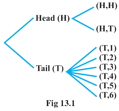
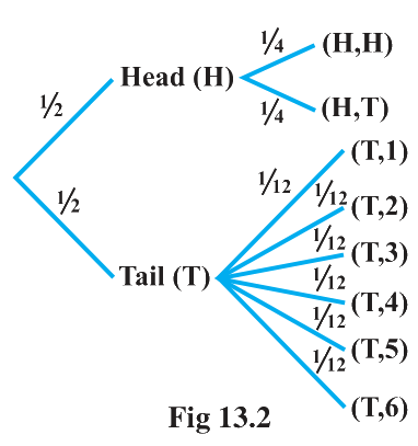
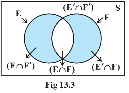
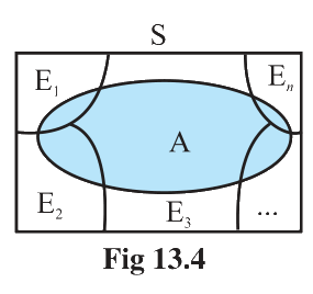
Fig 13.1: the tree diagram for a coin toss followed by a second stage, with the possible outcomes listed on the branches.