

Concepts: dispersion, range and mean deviation
Statistics24 min readLesson 2 of 6
2.1 Why the mean is not enough
Consider two batsmen with the same average. Batsman P scores 10, 90, 20, 80, 30, 70, 40, 60, 50 and 50, while batsman Q scores 45, 48, 50, 52, 55, 49, 51, 47, 53 and 50. Both have a mean of 50, so a single average cannot separate them. Their ranges do: P's scores run from 10 to 90, a spread of 80, while Q's scores run from 45 to 55, a spread of only 10. Q is consistent and P is erratic. The dispersion of data measures this scatter, and it is the second number needed to describe a data set after its central value. Two data sets with equal means can differ in spread, and ignoring spread can lead to wrong decisions, for example when choosing a bowler for a tournament or a machine for a factory.
Slideshow, slide 1 of 4. Use the left and right arrow keys to change slides and the space bar to play or pause.


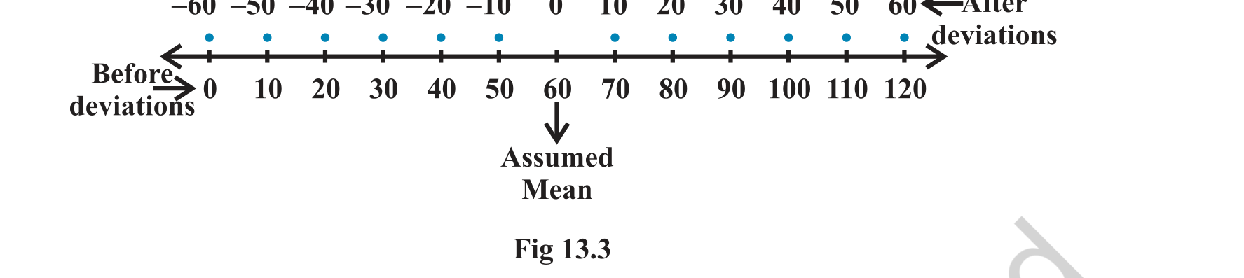
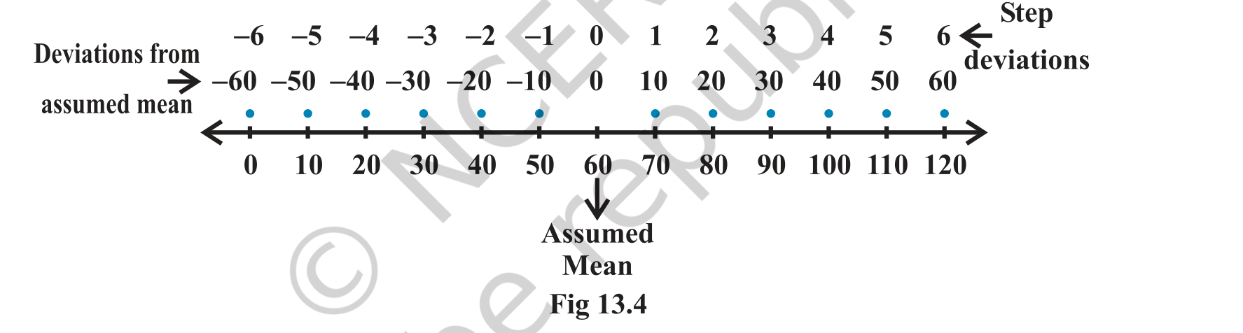
NCERT Figure 13.1: runs scored by batsman A shown as dots on a number line, spread across a wide range.
2.2 Range
The range is the difference between the largest and the smallest observation: range = maximum minus minimum. For the two batsmen above, the ranges are 80 and 10. The range is easy to compute and easy to understand, and it is useful for quality control where we need to know how far a measurement can drift. Its weakness is that it uses only two observations. A single extremely large value or a single extremely small value can change the range a great deal while the rest of the data stay the same. For example, the scores 45, 48, 50, 52 and 55 have range 10, and the set 45, 48, 50, 52 and 90 has range 45, even though much of the data is similar.
2.3 Mean deviation about the mean
The mean deviation measures how far the observations are from a central value on average. First find the mean, then take the absolute value of each deviation from the mean, and average those absolute deviations. The absolute value is needed because the deviations themselves add up to zero when the central value is the mean. For n observations, the mean deviation about the mean is the sum of the absolute deviations divided by n. For a frequency distribution, each absolute deviation is multiplied by its frequency and the sum is divided by the total frequency N. For grouped data, the class mark, which is the mid-point of the class, replaces the observation. The same recipe works about the median, and the median may be preferred when the data contain extreme values because it is less affected by them.
2.4 Worked example: mean deviation about the mean
Take the data 6, 8, 10, 12, 14, 16 and 18. The mean is 12, because the values are symmetric about 12. The deviations from the mean are minus 6, minus 4, minus 2, 0, 2, 4 and 6. Their absolute values are 6, 4, 2, 0, 2, 4 and 6, whose sum is 24. There are seven observations, so the mean deviation about the mean is 24/7, which is about 3.43. The mean deviation has the same units as the data. An average difference of 3.43 from the mean tells us the scores typically sit between about 8.5 and 15.5.
2.5 Mean deviation for grouped distributions
When the data are given with frequencies, we form a table with three columns: the value or mid-point, the frequency, and the weighted absolute deviation. The total of the third column divided by the total frequency is the mean deviation. The same table also gives the median when the cumulative frequencies are tracked. For a continuous distribution, the median class is the class whose cumulative frequency reaches N/2, and the median is found by interpolation inside that class. The calculation of mean deviation then uses the mid-points of the classes, which is an approximation because the individual observations inside a class are not known.
2.6 Choosing a central value
For the mean deviation, the centre can be the mean, the median or the mode, and the three choices give different numbers for the same data. The mean is convenient because it uses all the observations, but it is pulled by extreme values. The median is robust: a single very large observation moves it only slightly, so the mean deviation about the median changes less when one reading is doubtful. In a symmetric data set the mean and the median are equal and the choice does not matter. In a skewed set, such as household incomes where a few very rich households stretch the right tail, the median is the better centre. Exam questions state which centre to use, so read the instruction carefully before starting the table.
2.7 Limitations of the mean deviation
The mean deviation has two practical weaknesses. First, it uses absolute values, and the absolute value function is not smooth at zero, so the mean deviation is hard to handle algebraically; it cannot be split into independent contributions the way squared deviations can. Second, when the variability is very high, the median may not be a representative centre, and a mean deviation about such a median can be misleading. For these reasons the variance and the standard deviation, built from squared deviations, are the standard measures in statistics. The mean deviation remains useful as a quick descriptive number and appears in many textbook questions.
Tip
Always write the deviations in a table when the data are grouped. A single arithmetic slip in one row changes the mean deviation and the variance together, and the table makes that slip easy to spot.