

Concepts: variance, standard deviation and grouped data
Statistics24 min readLesson 3 of 6
3.1 From absolute deviations to squared deviations
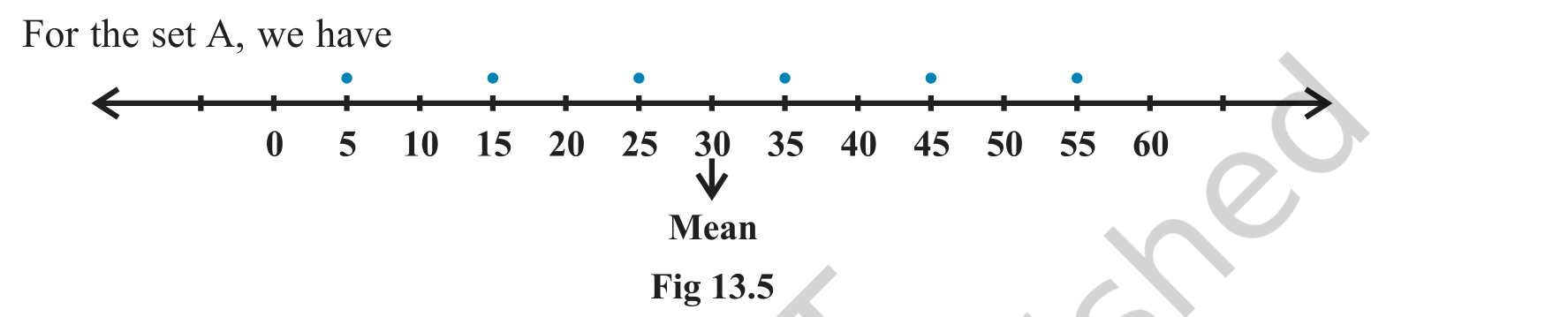
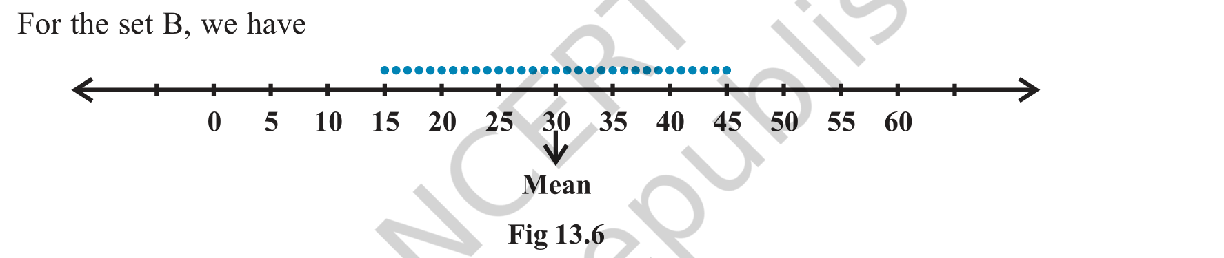
Imagine two sets of numbers with the same mean. Set A has six numbers spread far apart, while set B has ten numbers packed in a narrow band around the same mean. If we add the squared deviations from the mean, set A gives a larger total, but the total also grows with the number of observations, so comparing the sums is unfair. Taking the average of the squared deviations removes that dependence on the number of observations, and the resulting number is called the variance. Its square root, the standard deviation, has the same units as the data and is easier to interpret. Variance is denoted by sigma squared and standard deviation by sigma.
3.2 Variance and standard deviation for ungrouped data
For n observations with mean x bar, the variance is the sum of the squared deviations divided by n. The deviation is squared so that positive and negative deviations cannot cancel. Because every term is non-negative, the variance is zero only when every observation equals the mean, which is the case of no dispersion at all. In the calculation, the mean is computed first, then each deviation is squared, then the squares are added and divided by n. The standard deviation is the positive square root of the variance. A small standard deviation means the observations are tightly clustered; a large one means they are widely scattered. Unlike the variance, the standard deviation is expressed in the original units, so a standard deviation of 5 marks means typical distances of about 5 marks from the mean.
3.3 Worked example: variance of ungrouped data
Take the five observations 4, 8, 12, 16 and 20. Their mean is 12. The deviations are minus 8, minus 4, 0, 4 and 8, whose squares are 64, 16, 0, 16 and 64. The sum of the squares is 160, so the variance is 160/5 = 32 and the standard deviation is the square root of 32, which is about 5.66. If each observation were doubled, the new observations would be 8, 16, 24, 32 and 40, the deviations would double, the squares would become four times as large, and the variance would become 128. Doubling the data multiplied the variance by four and the standard deviation by two.
3.4 Worked example: variance from a frequency table
Take the values 4, 6, 8 and 10 with frequencies 1, 2, 3 and 4. The total frequency is 10 and the weighted sum is 4 + 12 + 24 + 40 = 80, so the mean is 8. The deviations are minus 4, minus 2, 0 and 2, whose squares are 16, 4, 0 and 4. Weighting the squares by the frequencies gives 16 + 8 + 0 + 16 = 40, so the variance is 40/10 = 4 and the standard deviation is 2. Notice that the frequency of the value 8 is irrelevant to the squared-deviation sum because that value sits exactly on the mean; frequencies matter only for the values away from the centre.
3.5 Discrete and continuous frequency distributions
When the data come with frequencies, each squared deviation is weighted by the frequency of its value, and the sum is divided by N, the total frequency. For a continuous distribution the classes are replaced by their mid-points, and the same weighted formula is used. This replacement is an approximation, because the observations inside a class are assumed to sit at the mid-point. For a wide class the approximation is coarser, which is why statisticians prefer narrow classes when the raw data are not available.
3.6 The variance as an average
The variance is an average, so it does not grow simply because a data set is larger. Doubling the number of observations by repeating the same values leaves the variance unchanged, while adding a single wild value can raise it sharply because the squared deviation of that value enters with full weight. This sensitivity is why a data set with one outlier can show a large standard deviation even when most observations are close together. A box plot or a stem plot is a useful companion to the numerical summary for exactly this reason. In an exam, report the variance and the standard deviation together, because the variance alone does not show the scale of the original data.
3.7 Worked example: grouped data
Consider five classes with mid-points 15, 25, 35, 45 and 55 and frequencies 2, 3, 5, 4 and 1. The total frequency is 15 and the weighted sum of the mid-points is 30 + 75 + 175 + 180 + 55 = 515, so the mean is 515/15 = 34.33. The deviations are minus 19.33, minus 9.33, 0.67, 10.67 and 20.67, and their weighted squares give a variance of about 152.5 after division by 15. The standard deviation is about 12.35. The arithmetic is heavy, which motivates the shortcut method with an assumed mean and step deviations.
Common mistake
Do not forget to divide by N when you compute the variance of a frequency distribution. The sum of the weighted squared deviations alone is not the variance; it is N times the variance.