

Exercise practice: Motion in a Straight Line
Motion in a Straight Line24 min readLesson 4 of 6
4.1 Exercises 2.1 to 2.4: describing motion
Exercise 2.1 asks when a body can be treated as a point object. A railway carriage moving between two stations qualifies because the distance is far larger than the carriage. A monkey sitting on a moving cycle does not qualify for a study of the monkey's own motion, since its size matters to what is being described. A spinning cricket ball and a tumbling beaker also fail, because their rotation and shape are part of the motion.
Exercise 2.2 reads two position-time graphs of children walking home from school. The child whose graph ends at a smaller position lives closer. The earlier start is the graph that leaves the origin first. Walking faster means a steeper slope. The same finishing time shows both reach home together. A crossing point means one child overtakes the other, and a single crossing is the usual answer.
Exercise 2.3 asks for the position-time graph of a woman who walks 2.5 km to her office in half an hour, stays there from 9.30 am to 5 pm, and returns by auto in six minutes. Most of the graph is a horizontal segment for the stay, with a gentle positive slope for the walk and a steep negative slope for the return. Exercise 2.4 tracks a drunkard who moves 5 steps forward and 3 back, one step per second, and the graph shows the sawtooth pattern from which the pit at 13 m is reached at 29 s.
4.2 Exercises 2.5 to 2.10: equations, throws and averages
Exercise 2.5 is the braking car. With u = 35 m s^-1, v = 0 and x = 200 m, the retardation is about 3.06 m s^-2 and the stopping time about 11.4 s. Exercise 2.6 throws a ball up at 29.4 m s^-1 and asks for the direction of acceleration on the way up, which is downward throughout. At the highest point the velocity is zero and the acceleration is 9.8 m s^-2 downward. Setting the top as the origin with downward positive gives positive position, velocity and acceleration after the top, and the ball rises 44.1 m and returns after 6 s.
Exercise 2.7 lists statements to judge. A particle with zero speed at an instant can have non-zero acceleration, a ball at the top proves it. A particle with zero speed has zero velocity, since speed is the magnitude of velocity. Constant speed does not imply zero acceleration, because a change of direction means a change of velocity. Positive acceleration does not imply speeding up, because the velocity may be negative.
Exercise 2.8 asks for the speed-time graph of a ball dropped from 90 m that loses one tenth of its speed at each bounce. The first fall takes about 4.3 s and the first impact speed is about 42 m s^-1, so the rebounds shorten in a geometric pattern. Exercise 2.9 explains why the magnitude of displacement never exceeds the path length and why the magnitude of average velocity never exceeds the average speed, with equality when the motion never reverses. Exercise 2.10 asks for average velocity and average speed over three intervals and shows that on the return leg the average velocity can be zero while the average speed is not.
4.3 Exercises 2.11 to 2.14: graphs and relative velocity
Exercise 2.11 asks why instantaneous speed equals the magnitude of instantaneous velocity. Over a vanishingly small interval the body cannot reverse direction, so the path length and the magnitude of displacement become the same number in the limit. Exercise 2.12 shows four graphs and asks which cannot describe one dimensional motion. A position-time graph cannot double back on itself, because the body would have two positions at one instant, and a velocity-time graph must remain single valued for the same reason.
Exercise 2.13 displays a position-time graph that is a straight line for negative time and a parabola after, and asks whether the particle moves along a straight line and then along a parabolic path. It does not: the graph plots position against time, not the path in space. The particle still moves along one line, and the graph is exactly what a body at rest before t = 0 and then uniformly accelerated would produce, for example a ball released from rest with a small initial position.
Exercise 2.14 is the police van and the thief's car. The van moves at 30 km h^-1 and the car at 192 km h^-1, so their relative speed is 162 km h^-1, equal to 45 m s^-1. The bullet leaves the van at 150 m s^-1 relative to the van, so its ground speed is about 158 m s^-1. The speed at which it approaches the thief's car is 158 - 53.3, about 105 m s^-1. The damage is done by the relative speed, which is the answer the question asks for.
4.4 Exercises 2.15 to 2.18: reading graphs
Exercise 2.15 asks for a physical situation matching four given graphs. A graph that rises, stays flat and falls can be a person walking, resting and walking back. A graph that is a horizontal line above the axis is motion at constant speed. A velocity-time graph that crosses the axis describes a body that reverses direction, such as a ball thrown upward. The exact story is less important than matching each graph's slopes and signs to a real motion.
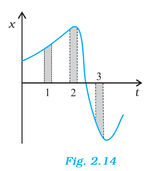
Exercise 2.16 reads a position-time graph of simple harmonic motion and asks for the signs of position, velocity and acceleration at three instants. At a positive position with the curve falling, the velocity is negative and the acceleration points back toward the origin, so it is negative as well. Exercise 2.17 compares three equal time intervals on a position-time graph. The interval with the steepest slope has the largest average speed, the flattest has the smallest, and the sign of the average velocity follows the direction of the displacement.
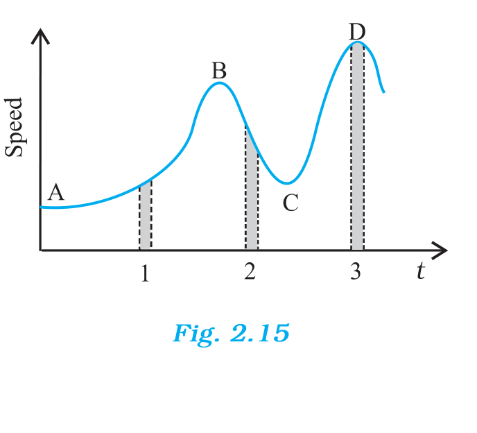
Exercise 2.18 uses a speed-time graph. The interval with the steepest slope has the largest average acceleration, and the interval with the highest average height has the largest average speed. The acceleration at a point is the slope of the tangent there, so the points where the curve is flat have zero acceleration. The figures below are the graphs from these exercises.
Slideshow, slide 1 of 3. Use the left and right arrow keys to change slides and the space bar to play or pause.
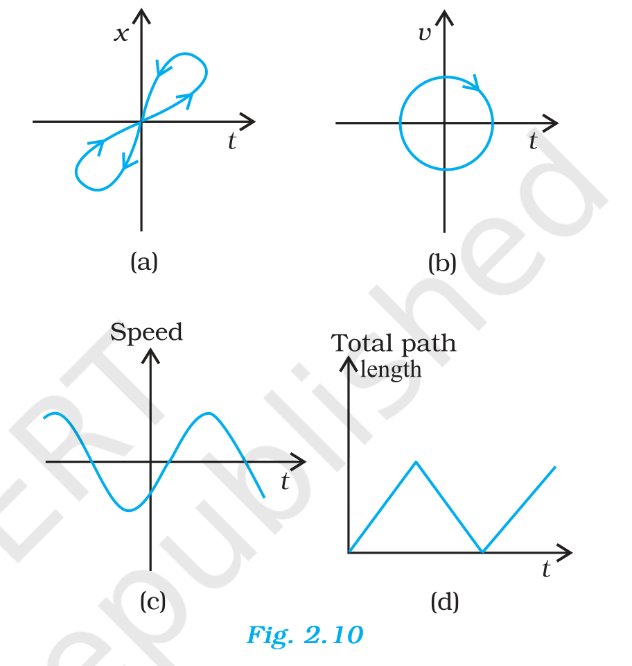
NCERT Figure 2.10: four candidate position or velocity graphs from exercise 2.12, used to test which cannot describe one dimensional motion.