Concepts: Population growth models

2.1 Four processes change a population

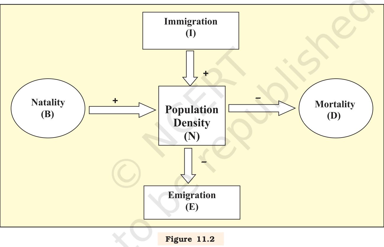
The size of a population never stays still. Food supply, predation and bad weather all push it up or down, and the changes in density are what tell us whether a population is doing well. Four basic processes are responsible. Two add individuals and two remove them.

Natality counts the births over a set period, added to the density at the start. Mortality counts the deaths in that same period. Immigration counts same-species individuals entering the habitat from outside. Emigration is the number that leave the habitat for somewhere else.

If N is the density at time t, then the density at time t+1 is written as Nt+1 = Nt + [(B + I) - (D + E)]. The population grows when births plus immigrants exceed deaths plus emigrants. Births and deaths usually dominate; immigration and emigration matter mostly in special cases, such as a new habitat being colonised, where arrivals can add more than births do.

2.2 Exponential growth

When food and space are unlimited, a species can realise its full innate capacity to increase, which is the point Darwin made when he built the idea of natural selection. Growth then follows an exponential pattern.

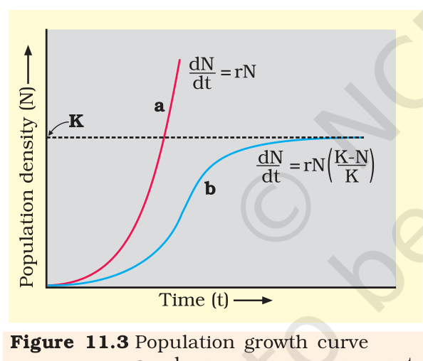
Let b be the per-capita birth rate and d the per-capita death rate. The change in N per unit time is dN/dt = (b - d)N. Writing r for (b - d) gives dN/dt = rN. The constant r is the intrinsic rate of natural increase, a key number for judging how a biotic or abiotic factor affects growth. For values, the Norway rat has r = 0.015 and the flour beetle 0.12; the human population of India had r = 0.0205 in 1981. The integral form of the equation is Nt = N0 e^(rt), where e is the base of natural logarithms, about 2.71828. Plotted against time, N gives a J-shaped curve (Figure 11.3).

The chessboard story makes the size of exponential growth concrete. A minister asked for one grain of wheat on the first square, two on the second, four on the third, doubling each time. The king agreed without thinking, and by the time half the board was covered all the wheat in his kingdom would not have finished the job. A single Paramecium doubling daily would reach a similar surprise in 64 days if food and space never ran out.

2.3 Logistic growth

No population in nature has endless resources, so exponential growth cannot go on. Limited resources bring competition between individuals, and the fittest survive and reproduce. Every habitat has an upper limit to the number it can support, and growth stops once that number is reached; this ceiling is the carrying capacity, K.

In a habitat with finite resources a population passes through a lag, then speeds up, then slows, and finally settles at K. The resulting plot of N against time is a sigmoid curve (Figure 11.3). This is the Verhulst-Pearl logistic growth, described by dN/dt = rN(K - N)/K. Here N is the density at time t, r the intrinsic rate of natural increase and K the carrying capacity. Since resources are finite for most animal populations, the logistic model is the more realistic of the two.

2.4 Life history variation

Populations evolve to maximise reproductive fitness, also called Darwinian fitness, which means a high r in the habitat where they live. Under a given set of selection pressures, organisms move towards the most efficient reproductive strategy.

Some breed once in a lifetime, such as the Pacific salmon and bamboo; others breed many times, which most birds and mammals do. Some produce many small offspring, as oysters and pelagic fishes do; others produce a few large offspring, as birds and mammals do. Neither pattern is universally better. Ecologists explain life history traits as having evolved in response to the abiotic and biotic constraints of the habitat, and this remains an active area of research. The two growth models are not rivals but tools with different uses. The exponential model describes what a population could do if nothing held it back, which is useful in the early stage of a colonising species or in the laboratory. The logistic model describes what usually happens in the field. Neither model says anything about age structure, migration or the details of the habitat. Ecologists read them as first approximations and then add the biology the equation leaves out. A population that starts below K grows quickly at first, and the same population slows as it approaches K because the per-capita growth rate itself falls.