Concepts: potential, potential difference and the potential of a dipole

Electrostatic Potential and Capacitance22 min readLesson 2 of 7

2.1 Why a potential can be defined The electrostatic force is conservative, so the work done in moving a charge between two points depends only on the endpoints and not on the path taken. That is the property that lets us assign a single number, the potential, to every point in space. The reference point is taken at infinity, where the potential is set to zero. The potential at a point tells how much work an external agent spends per unit positive charge to carry a small test charge there from infinity, moving it slowly. The test charge is moved without gaining speed, so the agent's work goes into the field configuration rather than into kinetic energy. Potential difference between two points is the work per unit charge in moving between them. It is measured in volt, and one volt equals one joule per coulomb. The field and the potential difference are linked: moving with the field lowers the potential, and moving against the field raises it. 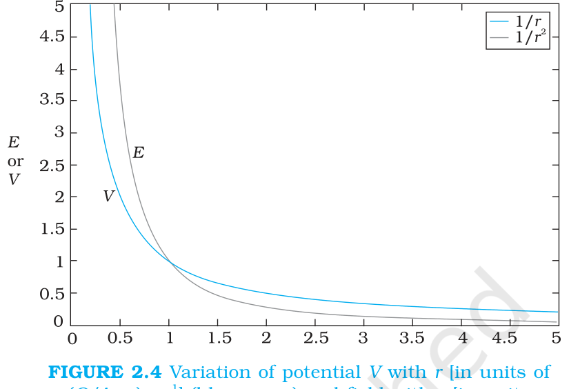2.2 Potential due to a point charge Take a charge Q at the origin and bring a test charge from infinity to a distance r. The field falls as one over the square of the distance, and integrating that force over the path gives a potential that falls as one over r. The sign follows the charge: a positive charge gives a positive potential everywhere, and a negative charge gives a negative potential. The potential around a positive charge is largest close to it and tends to zero at large distances. A negative charge has the lowest potential close to it and rises toward zero at infinity. The field points downhill, that is, from higher potential to lower potential, in both cases.

Graphs of potential V against distance r and electric field E against distance r for a point charge, showing V falling as one over r and E falling as one over r squared.

V (r) = \frac{1}{4 π ε _{0}} \frac{Q}{r}

Potential due to a point charge, with V = 0 at infinity

W_{Q \to P} = q (V_{P} - V_{Q}) = - q \int_{Q}^{P} E \cdot d l

Work done on a charge moved between two points

Geometry used to calculate the potential at a point due to an electric dipole, showing the distances from the point to the two charges and the angle of the position vector.

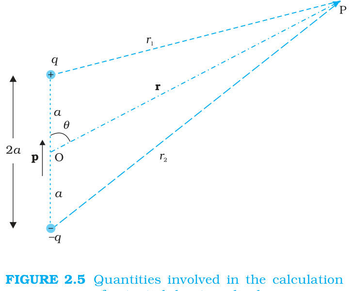
2.3 Potential due to a dipole A dipole is a pair of charges +q and -q separated by a distance 2a. At a point far from the pair, the two potentials nearly cancel and what survives depends on the angle between the position vector and the dipole moment. On the axis the potential is large and positive on the side of the positive charge; on the equatorial plane it is exactly zero, because the point is equidistant from the two charges and their potentials cancel. At a distance r much larger than a, the potential of a dipole falls as one over r squared. Compare this with the field of a dipole, which falls as one over r cubed. The angle enters the potential through cos theta, where theta is measured from the dipole moment. For a collection of charges, the potential at a point is the algebraic sum of the individual potentials. A positive and a negative charge close together give a small net potential at far points, which is why the dipole result falls faster than the point charge result. 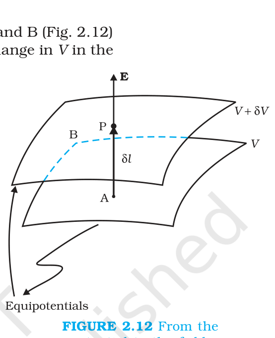2.4 Relation between field and potential The field is the negative gradient of the potential. In one dimension that means the field equals minus the slope of the potential distance graph. A steeply falling potential means a strong field, and a region where the potential is constant has zero field. This relation gives a quick check on every potential curve you meet in this chapter. For a uniform field the potential falls linearly with distance along the field, and equipotential surfaces are planes perpendicular to the field. For a point charge the potential varies as one over r and the equipotential surfaces are spheres.

V_{dipole} = \frac{p cos θ}{4 π ε _{0} r ^{2}} (r ≫ a)

Potential of a dipole at a far point; zero on the equatorial plane

Diagram showing how the electric field is obtained from the potential, with the field pointing from higher to lower potential and equal to the negative gradient of V.

Warning

Potential is a scalar and can cancel to zero at a point where the field is not zero. At the midpoint between equal positive charges the field is zero but the potential is twice the potential of one charge. Keep the two ideas separate in the answer.

2.5 Worked example: potential of two charges A charge of 1 microcoulomb is at the origin and a charge of -2 microcoulomb is 30 cm to its right. Find the potential at a point 10 cm to the right of the positive charge. The point is 0.1 m from the positive charge and 0.2 m from the negative one. The two potentials are k q1 / r1 = 9 \times 10^4 V and k q2 / r2 = -9 \times 10^4 V. Their sum is zero, so this point has zero potential while the field there is not zero. That is the scalar cancellation that makes potential problems easier than field problems.

2.6 Sign conventions worth fixing early Potential is positive near a positive charge and negative near a negative charge when infinity is the zero. Moving a positive charge toward a positive source increases its potential energy, and moving it toward a negative source decreases it. The field always points from higher potential to lower potential, so a positive charge drifts the same way as the field and a negative charge drifts against it. Write the signs on the diagram before using the formulas; most sign errors in this chapter come from skipping that step.

in hinglish

Potential ka matlab ek unit positive charge ko infinity se point tak laane mein kiya gaya kaam. Kyunki electrostatic force conservative hai, yeh kaam path par depend nahi karta, isliye har point ko ek potential de sakte hain. Potential difference do points ke beech ka work per unit charge hai, aur unit volt hai. Point charge ka potential k Q / r hota hai, field 1 / r^2 se girta hai par potential 1 / r se girta hai. Dipole ka potential far point par p cos theta / 4 pi epsilon nought r^2 hota hai, aur equatorial plane par zero hota hai. Potential scalar hai, isliye charges ke potentials seedha add hote hain, vector nahi banana padta. Field aur potential ka rishta E = -dV/dr hai: jahan potential jaldi girti hai wahan field strong hoti hai. Yaad rakho, potential zero ho sakta hai aur field zero na ho, aur field zero ho sakti hai aur potential zero na ho.