xSkill: notes, lectures and practice for CBSE and CSE

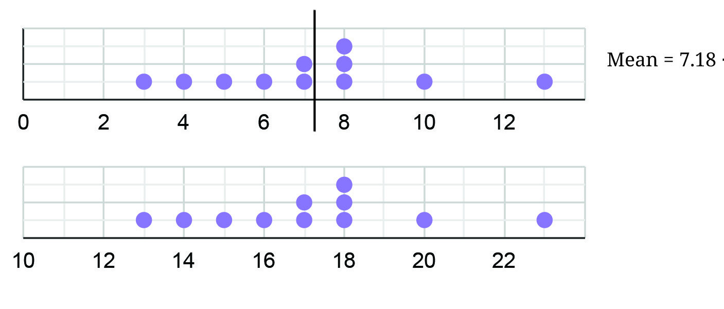
1.1 Mean as the balance point The mean of a collection shares its total equally among the values: add all the values, then divide by how many there are. In earlier classes we saw the mean as a fair share. This chapter looks at it as a balance point. Draw the values as dots on a number line. The mean is the point where the total distance of the dots on its left equals the total distance of the dots on its right. For the pair 3 and 7, the mean is (3 + 7) \div 2 = 5, exactly halfway between them. For 8 and 9 the mean is 8.5, again halfway. With more values the mean need not sit at the midpoint of the smallest and largest values. For the collection 10, 10, 11 and 17 the mean is 12, and the two 10s are 2 units below it while the 11 is 1 below and the 17 is 5 above. The total below is 2 + 2 + 1 = 5 and the total above is 5, so the mean balances the collection. There is only one such balance point. If you try a value to the right of the mean, all the left distances grow and all the right distances shrink, so the two totals no longer match. A value to the left fails for the same reason in the other direction.

mean = \frac{x _{1} + x _{2} + \dots + x _{n}}{n}

Mean of n values

left \sum (mean - x_{i}) = right \sum (x_{i} - mean)

The mean balances the distances on both sides

1.2 Median as the middle value The median is the central value once the data has been put in order. When the number of values is odd, the median is the middle value itself. When the number of values is even, the median is the average of the two middle values. The median splits the data into two halves with the same number of values, though not necessarily the same total distance. Both measures describe the centre of data but they react differently to changes. The mean uses every value, so one very large or very small value can pull it a long way. The median depends only on the middle positions, so it is more stable against a few extreme values. Choosing between them depends on the question: a fair total points to the mean, while a typical middle value points to the median.

\text{median}=\text{middle value \left(odd count\right)} \qquad \frac{a+b}{2}\ \text{\left(even count\right)}

Median for odd and even counts

1.3 Mean and median from a frequency table When values repeat, a frequency table is shorter than writing every value. The mean then uses each value as many times as its frequency: multiply every value by its frequency, add those products and divide by the total frequency. The family-size data takes the values from 3 up to 10. The matching frequencies are 3, 11, 9, 7, 3, 1, 1 and 1, so there are 36 families and the values add to 188; the mean family size is 5.22. For the median, the cumulative frequencies tell us where the middle positions fall. The 18th and 19th values of 36 lie after the frequencies of 3 and 4 add to 14 and before 3, 4 and 5 add to 23; all positions from 15 to 23 hold the value 5. So the median family size is 5. This is much faster than writing all 36 numbers.

frequency mean = \frac{\sum f _{i} x _{i}}{\sum f _{i}}

Mean from a frequency table

1.4 Reading a line graph in two steps A line graph joins data points with line segments, so it is best for showing change over time. When you meet one, follow a two-step process. First identify what is given: read the title, the labels of both axes, the scale and the shape of each line. Second infer and interpret: describe the trend, compare the lines, locate peaks and lows, and make statements that the graph actually supports. A grouped column graph can also show the same data, but with many time points it becomes crowded. Line graphs stay readable because a line carries the eye through the trend. The chapter uses them for temperatures, rainfall, births, lighting sources, hobbies, sunrise and sunset times, and the lunar cycle. The next page practises the reading method, and the exercise pages apply it to graphs with real data.

point on a line = (value on horizontal axis, value on vertical axis)

How to read a point on a line graph

1.5 Choosing between mean and median Use the mean when every value should count towards a total, such as an average score or a fair share. Use the median when a few extreme values would distort the picture, such as house prices or waiting times. A single very large value can move the mean a long way while leaving the median untouched. A good report often gives both, because together they warn the reader when the data has a skew. The mean of counting data need not be a counting number: a family-size mean of 5.22 families is perfectly meaningful. The median of the same data must be an actual value or halfway between two values. Keeping that difference in mind prevents the mistake of rounding a mean to a nearby data value and presenting it as if it were observed.